By GUPPI
You have heard about reinforcement learning for next best action optimization but don't really know why you would use it over other techniques or how to use it best?
In this article, we try to demystify and explain how we used offline reinforcement learning to have a good baseline model for optimizing marketing campaigns.
A quick recap
As mentioned in the initial post of this series, the baseline logistic regression model had many drawbacks when recommending a next best action: it could not incorporate the future, could not leverage the sequential nature of the data, could not recommend an optimal sequence of actions nor could it adjust automatically to changing environment dynamics. That is the reason why we introduced reinforcement learning as our lifesaver. In this blog post, we will go into more details as to why reinforcement learning could help us and how we actually implemented this.
Why reinforcement learning?
As the nature of a next best action recommendation problem is sequential, this means that the problem can be modeled as a Markov Decision Process (MDP) and solved by reinforcement learning methods. In a MDP, there is an agent interacting with an environment. This agent chooses an action and observes what happens in the environment after it took the action. Then, it receives a reward in correspondence with the action and the state it transitioned to. The agent repeats the interaction many times and learns what action is optimal at each state.
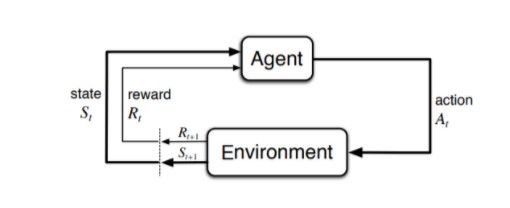
The advantages that reinforcement learning (RL) based recommenders have over traditional recommenders are twofold. First, RL-based recommenders can consider this sequential nature in contrast with the more traditional methods (such as collaborative filtering). They can hence be developed to optimize the long-term reward (instead of the immediate reward) with the added benefit that these methods can be tweaked as to how much importance they will give to future rewards. Indeed, one of the most important hyperparameters to tune in reinforcement learning is 𝜸, the discount factor. The discount factor in essence determines how much importance the agent will assign to future rewards. With 𝜸 being 0, the agent will only consider immediate rewards and will be completely myopic. With 𝜸 being 1, all the rewards (immediate or distant) will be weighed equally. Second, when deployed in an online fashion, agents receive direct feedback and can flexibly adapt themselves to better reflect the changing environment dynamics.
Methodology
First, we split the data into a train, validation and test set. All three sets contain the whole period/sequence of data (i.e. we consider the time sequence for building a MDP), but were split based on clients. This means that clients in the train set will not be present in the validation nor test set. We believe that in our case there will not be any data leakage since the timing of the campaign is not so important and as the features are pretty static.
We then needed to create a MDP dataset consisting of observations, rewards, terminals and actions.
- Observations = the features reflecting the state. To stabilize training, we performed PCA.
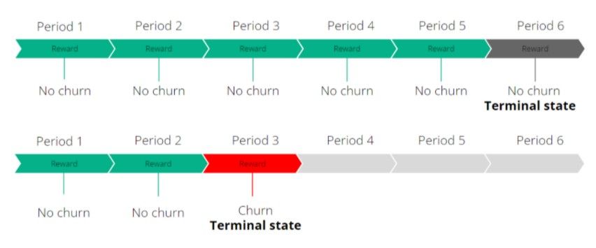
- Terminals = terminal state indicating the end of an episode. In our case, we considered customer churn as well as the end of the period as terminal states. This means that each customer sequence has a terminal state and will be an episode in itself.
- Actions = whether a campaign was targeted or not and by which campaign. This will be set to 0 if the client was not targeted by a campaign and will be set to the campaign number when that client was then targeted by that specific campaign.
- Rewards = feedback from the environment. We set the reward as -cost*action - target.
- The reward is the lowest when a campaign was targeted at a customer which then churned. This is a lose-lose situation as you wasted resources on targeting this customer who was about to churn anyway.
- The second lowest reward will be received in case when a customer churns and was not targeted by the campaign. That customer might have stayed if he was targeted by that campaign.
- The second highest reward will be handed out when a customer is targeted and did not churn.
- The highest reward is handed out when the customer did not churn and was not targeted by the campaign.
Choosing an algorithm
We used the d3rlpy library for reinforcement learning.
The algorithm used in the end was Discrete Conservative Q Learning which learns conservative value estimates by regularizing the Q values during training.
Two factors were crucial when picking the algorithm: it had to be specifically designed to handle offline reinforcement learning and it had to be able to handle discrete action spaces.
The first factor was essential since we only had a static, offline dataset available to train our model on. Consequently, no exploration of the policy is possible: there is no simulation environment available for the agent to interact with (in contrast to online learning).
However, this static nature poses a threat as well. Offline evaluation can be difficult since the new policy’s state-action visitation distribution may differ significantly from that of the behavior policy. This change in distribution as a result of policy updates is often referred to as a distributional shift and constitutes a major challenge in offline reinforcement learning. It is in general not possible to find the optimal policy in offline reinforcement learning, even when provided with an infinite sized dataset. Thus, the aim in offline reinforcement learning is to design algorithms that would result in a as low sub-optimality as possible
The second factor was necessary since our action space is discrete. Indeed, there are only a finite number of actions available, namely to not target or to target the customer with any of the campaigns considered.
Hyperparameters
In reinforcement learning, tuning the hyperparameters is also crucial. We experimented with the following hyperparameters:
- Alpha = penalty for out-of-distribution actions. As we work with an offline dataset, some state-action pairs will be underrepresented in the dataset as observations are quite limited in this space. This will result in high variance value estimates which this alpha hyperparameter tries to regularize. We observed that the higher this alpha parameter became, the less likely the reinforcement learning agent recommended sending out a campaign. This is likely due to the data being skewed more towards not sending out an action.
- N_steps = n-step TD calculation. The higher this number, the better the estimated future rewards will be.
- N_critics = number of Q functions for ensemble learning. The higher this number, the more accurate and stable the Q values will become.
- Gamma = discount factor. As previously explained, gamma will determine how much importance the agent will assign to future rewards.
Results
We will now show the results of the multi-campaign setting.
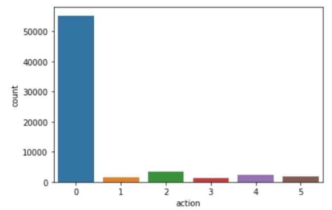
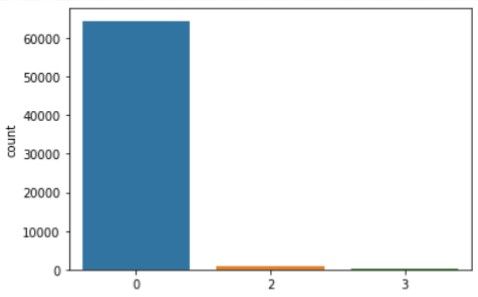
As one may notice when comparing figure 3 and figure 4, our reinforcement learning algorithm only recommends campaign 2 or campaign 3 (alongside recommending doing nothing). This may seem counterintuitive, but when analyzing the causal average treatment effects of the campaigns (cfr. figure 5), we perceive that indeed only campaign 2 and 3 were undoubtedly targeted at reducing churn.
In the end, our reinforcement learning model learned to recognize this behavior and hence only recommended action 2 and 3 (or no action). This is actually quite nice as this shows our model is robust against adding in bad campaigns. Even when adding these to the reinforcement learning algorithm, it seems to be able to disregard the bad campaigns and only select those having a valuable impact.

Currently, there is no standard for evaluating reinforcement learning offline. This is still an area of research. Usually, the model is then deployed and its performances are evaluated in a real life environment, where you can observe direct feedback from the customers. In many cases, it is very risky to deploy the model and let it recommend actions. Hence we evaluated the proposed Q-values from the model for different sets of actions. The Q-values are the estimations of your objective function, hence the higher the better. Since the setup is a bit more complex when adding in all the campaigns, we show below the results for only one campaign.
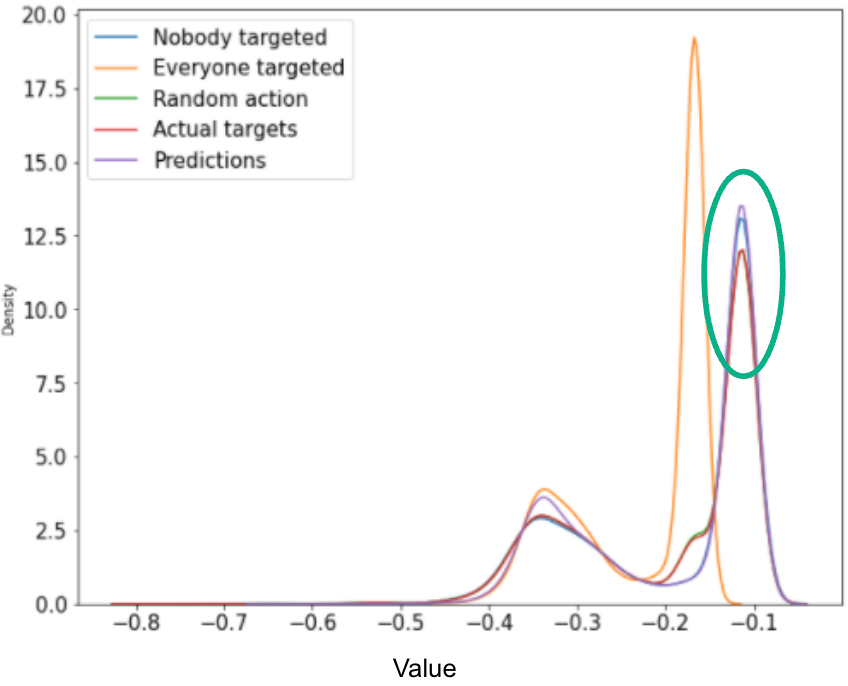
We observe that the model does estimate higher Q-values for the predicted actions and the values are slightly higher than if nobody was targeted. The model also recommends better actions than the actions proposed in the test set (actual targets).
Conclusion
To recommend a next best action, we used reinforcement learning as this approach has many advantages over the traditional methods that for instance cannot leverage the sequential nature of the data and cannot incorporate the future.
As we received a static, offline dataset, we had to ensure our reinforcement learning algorithm could handle this lack of exploration and interaction with the environment so as to alleviate the distributional data shift. Furthermore, it had to be able to handle a discrete action space. We chose discrete CQL for this end.
In the end, our reinforcement learning model seemed to only recommend two out of five actions. After further investigating this behavior, by running a causal inference analysis, we observed that indeed these two campaigns were the only ones clearly aimed at reducing churn. So, our reinforcement learning model learned to recognize the optimal campaigns and was robust to sub-optimal ones, recommending only the actions that were positively impacting churn.
Moreover, we noticed quite a large dependence of the algorithm's performance on its hyperparameters. By tuning these hyperparameters, better results could potentially be obtained.
Next steps?
Ideally, we should analyse the model for potential biases or unethical outcomes (and mitigate these if present). More business logic could be included in the reinforcement learning model (such as constraining the model to only recommend an action once a few months instead of consequently recommending an action.).
Once the model has been sufficiently stress tested, the next step would be to put the reinforcement learning model in a production environment. This means that the model will be able to actually recommend campaigns for certain customers (to the marketing team). Then based on the feedback generated from the campaigns, the model can be retrained, adapt itself and improve its performance.
Very important will be the trade-off between exploitation and exploration. Exploitation means that the RL agent will leverage and base its recommendations on the learned policy (the optimal decision based on the past observed data). Hence, it will leverage what it already knows. Exploration on the other hand allows the RL agent to randomly perform actions to gather new information to potentially improve its policy. Exploration will allow the RL agent to discover new and better ways of recommending actions.
Of course, when deploying a RL model, we preferably want to leverage past information and we do not want to start from scratch as it could be quite costly to randomly target customers (by for instance targeting those customers with a low probability to churn or those that will churn when targeted). On the other hand, by still allowing a small degree of exploration, the RL agent might improve its policy and might be able to adapt to changing customer preferences for instance. This tradeoff can be tackled by techniques such as epsilon-greedy, upper confidence bounds or Thompson sampling.
Work hard, play hard, dream big ?
The reinforcement paradigm allows for much more than just optimizing the customers to target and the right timing, you can envision to optimize basically anything. We could consider information such as price sensitivity, customer lifetime value etc. and hence propose campaigns that take this into consideration. An example could be to understand which customers will respond positively to a discount and how much the discount should be to get the optimal effect. Even dreaming further, we could have a RL agent that directly drafts the emails for the marketing team...

